Running the interactive workflow
The main way to use Resomapper is through a command-line interface (CLI), which allows users to easily follow the complete image processing pipeline. To use this CLI, after installing the package, simply open a terminal window and enter the resomapper_cli command.
> resomapper_cli
This will start the processing workflow, and if you need to stop it at any point, just press Ctrl + C. During this process, the user will be prompted to interact with the program via the terminal (writting a response and pressing Enter) or pop-up windows (clicking on different options).
The program will follow several steps:
1. Choosing a working folder
After displaying a welcome message in the terminal, a pop-up window will appear in which you’ll have to choose your working folder and press Select folder. This directory must contain all the studies we want to process, and it will also hold all the resulting files at the end (see Preparing the studies and Output filesfor more details).
Attention
Make sure that you have selected the correct working directory. If you are selecting the folder of only one study, it won’t be recognised. You should select the folder that contains that study (or more than one).
2. Converting studies to NIfTI
If your input data is not already on NIfTI format, the conversion of studies will automatically start after choosing the working directory. In case that the studies have already been converted and stored before on the same folder the user will be asked if they can be reused or they need to be converted again. When completed, a message will be shown. Also, the folders containing the converted studies will be labeled according to the BIDS format with the modal they contain for an easier identification afterwards. They will be stored under the working directory, inside a folder named resomapper_output (see SOURCEDATA: Converted studies).
3. Selection of modalities to process
The next step will be to select the modalities we want to process. Currently, in Resomapper, we have implemented the posibility to generate T1, T2, T2*, MTI and DTI parametric maps. A pop-up window will appear showing all these possibilities. You can check all the ones you want and press OK to start. For each study in the working directory, the selected modalities will be processed in case their adquisitions are present.

Modality selection window.
If any studies have already been processed and stored before, a message will be displayed in the terminal giving the option to process it again or not.
Attention
Take into account that processing it again means deleting any previous results for that modality (for the correspondig study). For that reason, make sure of copying them to another folder before continuing if you need them (you’ll recieve a warning message to remind you anyway).
At this point, the processing workflow for the several studies will start. A message will be shown in the terminal at the start of each study and for each modality inside of it.
4. Preprocessing the images
Before starting the processing, you will have the option to preprocess the images before generating the parametric map. Currently, the available preprocessing options available include several denoising filters, Gibbs artifact suppression and bias field correction.
For each of these, a question will be asked to determine if you want to use any of these, and if so, in the case of the denoising filters and bias field correction, a pop-up window will be shown asking for the filtering parameters. Usually, no changes should be done to these parameters, unless you get unwanted results and need to fine tune them.
After using any of the preprocessing options, a window will appear showing one of the slices of the original image and the corresponding preprocessed one. Also, in the case of the denoising filters or the Gibbs artifact correction, the residuals between both images (img1-img2)^2 will be shown. Ideally, in the case of denoising, these should be more or less randomly distributed, meaning that no structures of the original image have been over-smoothed. For Gibbs artifacts, you should see the removed rings in the residuals. In the case of the bias field correction, the calculated bias field will be shown. If you are not satisfied with the result, you can repeat the preprocessing as many times as you wish.
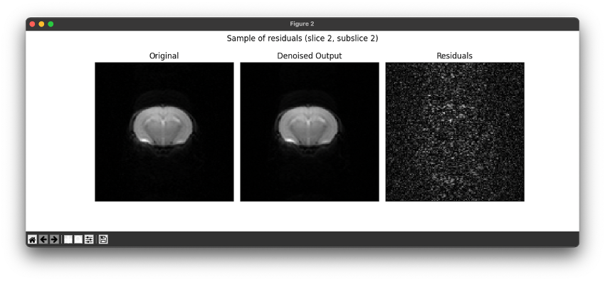
Filtered image pre-visualization.
5. Creating a mask
The first step for each instance will be to create the masks or ROIs (Region Of Interest) where we want the processing to take place (in the case of neuroimaging, we need to extract the brain). To do so, the user will be asked between the following options:
Selecting a file that contains a binary mask, in NiFTI format.
Reusing the last mask used for the current study. This option will be available only if any of the modals have been processed before and there is a mask file stored in the general study folder.
Manually creating a mask by drawing it. In this case, pop-up windows will be shown for each slice where the mask can be manually created following the steps shown in the terminal (left-clicking to create lines and right-clicking to close the outline).
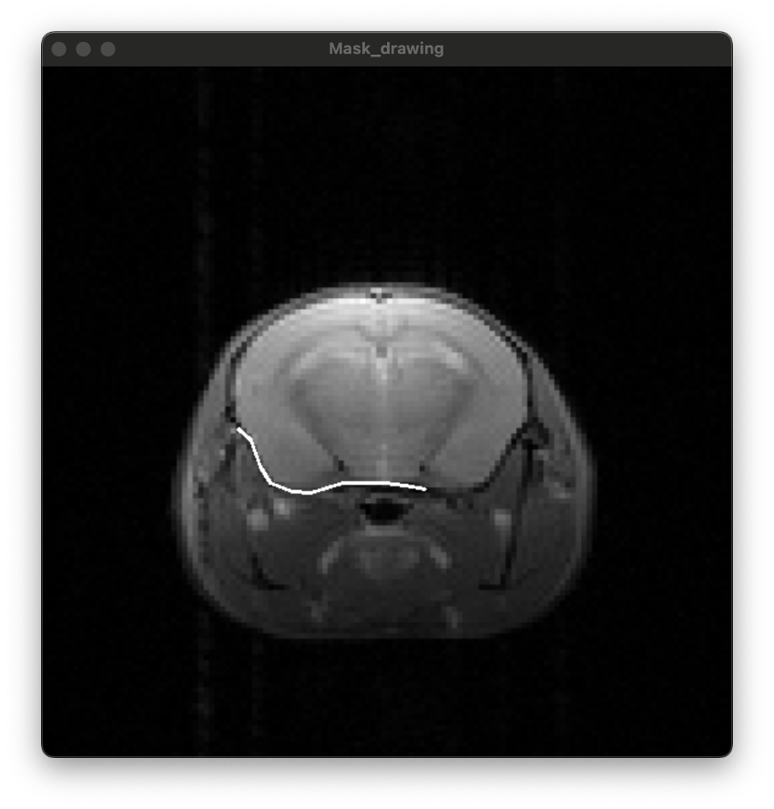
Manual mask creation.
After creating the masks for all slices, a pop-up window will appear with a preview of all of them. Once viewed the terminal will ask if it is correct. If you are not satisfied with the masks created, you can repeat the process as many times as necessary.
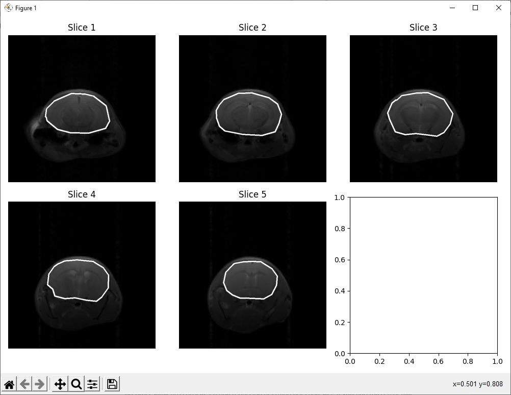
Mask pre-visualization window.
6. Processing
Once the previous steps have been completed, the processing of the corresponding modality will start. The workflow might vary a bit depending on the modality, as described in the following sections.
DTI - Diffusion Tensor Imaging
In this case, the user will first be asked for the diffusion weighted images acquisition parameters (number of b values, number of basal images and number of gradient directions).
This step is taken to help the user keep track of the adquisiton information. The parameter values introduced by the user will be checked with the adquisition method files of the study, and if any of them doesn’t match, the user will be warned. In the case of b values and the number of basal images, they will be automatically corrected.
However, in the case of the number of gradient directions, it may be the case that you want to remove some of the directions from the image because they were not acquired correctly. For this reason, if a number smaller than the real was specified, the user will be asked if that’s the number of directions desired instead. Anyways, if the correct number was introduced, the user will also be asked if any directions need to be removed, just in case. In both scenarios, after confirming the number of directions to be deleted, the index of those will be asked, as shown below.
Once we have confirmed all these adquisition parameters, the vector of effective b values and the directions matrix will be shown in the terminal.
Finally, the DTI model will be adjusted to the data. In total, the maps produced for this modality are:
ADC - Apparent Diffusion Coeficient
AD - Axial Diffusivity
RD - Radial Diffusivity
MD - Mean Diffusivity
FA - Fractional Anisotropy
Proccesing of DTI maps is made thanks to the DIPY library.
ADC for acquisitions of less than 6 directions
For DWI acquisitions with less than 6 directions available, the DTI model can’t be calculated. In that case, the program will provide the option to use the monoexponential decay model, that means fitting the signal values for each pixel to the following curve equation: \(S=S_0 * e^{-b * ADC}\)
There is also the option to do a line regression fitting to the linearized equation: \(ln(S)=ln(S_0) - b*ADC\)
The user will be given the option to choose between these two options, and then the model will be fitted. After that, the user will have the opportunity to examine the fitted curves for each pixel in an interactive graphic. Finally, the ADC map will be saved the same way as before.
Note
Fitting these models will only give the ADC map and the R2 map as outputs. AD, RD and FA maps are exclusive of the DTI model. MD can be estimated as the mean of all the ADC directions.
MTI - Magnetisation Transfer Imaging
In the case of MT images, no parameters need to be specified before the processing starts, but there might be several different images in the original study if we have modified the slope. If so, the program will ask which folder or folders we want to process (normally, folder 1 will be the original adquisition and the following ones will be the images with the modified slope). If there is only one folder, it will be processed directly. The processing of these images is very fast, because it does not require fitting the data to a model.
Relaxometry: T1, T2 and T2* maps
These maps do not require any additional specification before processing begins.
Processing of T maps is made thanks to the MyRelax library.
7. Saving the maps
Each time a map or a result is generated, in any of the modalities, a pop-up window will open showing the result. In addition, it will be possible to modify the color scale in which it is displayed, specifying the minimum and maximum value, as well as the name of the color palette.
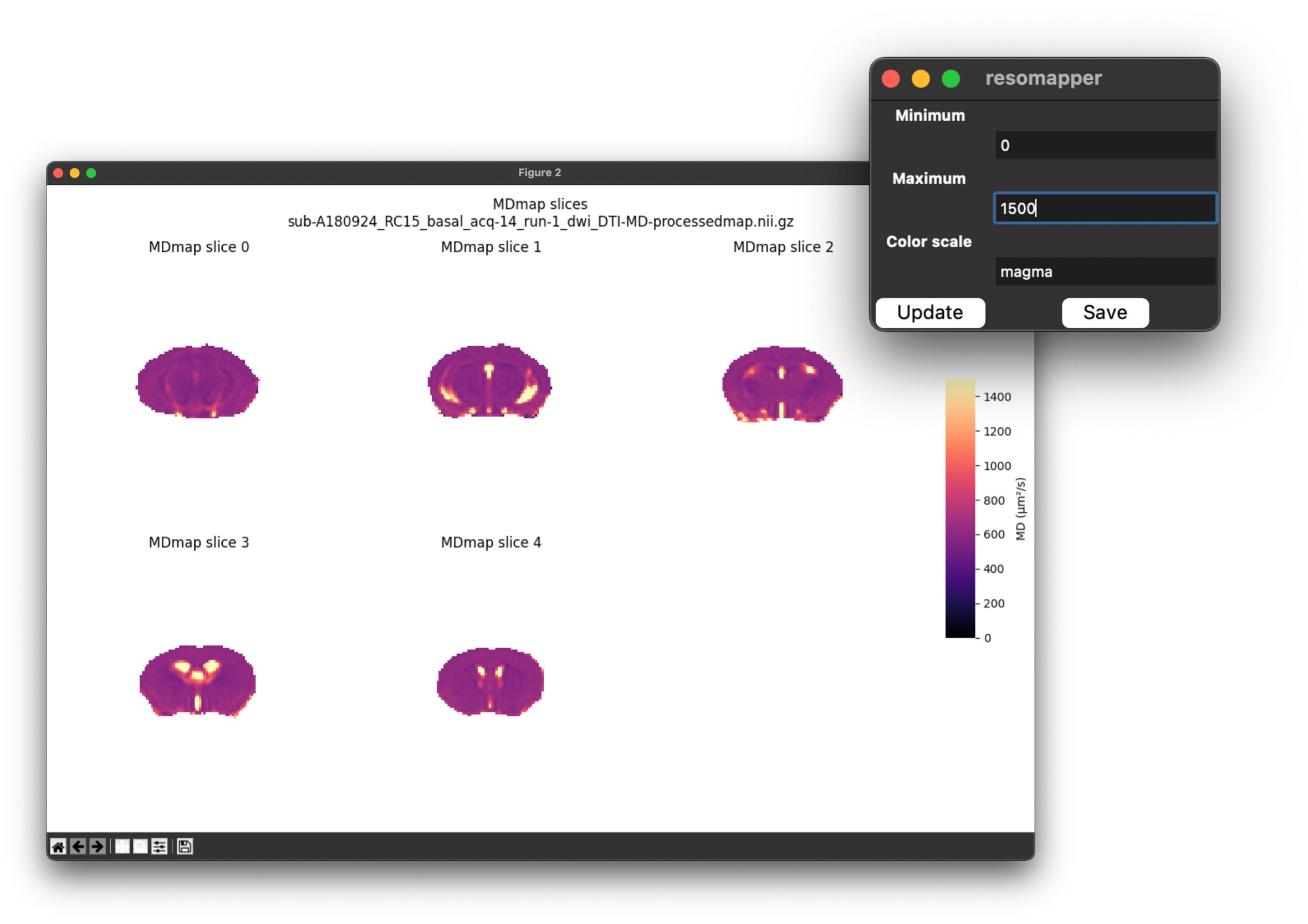
Map scaling windows.
The different color palettes and their names come from the Matplotlib package. You can use any of those, but in the figure below we show some of the most comon ones. You can try different combinations and visualize them by pressing the Refresh button. Once you are satisfied, click on Accept to save the map.
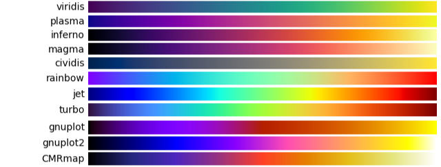
Different color palettes that can be used for map coloring.
When all the maps of the selected modalities from all the studies included in the working directory have been processed and, the processing will be complete and the Resomapper CLI will stop running.